1 Prepare datasets

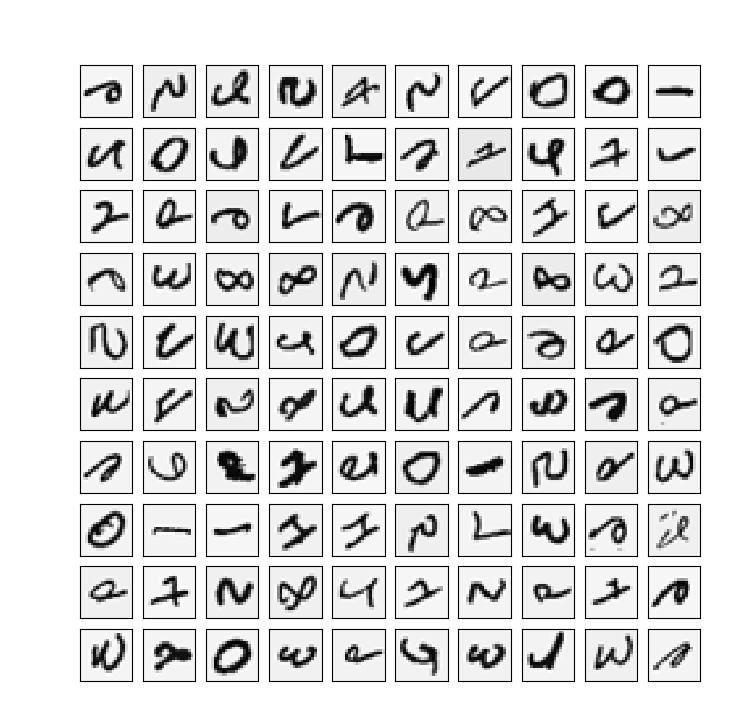
其中有5000个训练样本，每个样本是20*20像素的数字的灰度图像。每个像素代表一个浮点数，表示该位置的灰度强度。20×20的像素网格被展开成一个400维的向量。在我们的数据矩阵X中，每一个样本都变成了一行，这给了我们一个5000×400矩阵X，每一行都是一个手写数字图像的训练样本,预测手写数字图像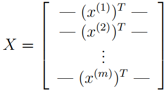

1.1 Visualizing the data 可视化数据

import numpy as np
import matplotlib.pyplot as plt
from scipy.io import loadmat
import scipy.optimize as opt
from sklearn.metrics import classification_report  # 这个包是评价报告
from sklearn.preprocessing import OneHotEncoder

'''
1.Prepare datasets
'''


def load_mat(path):
    '''
    读取数据
    :param path:
    :return:
    '''
    data = loadmat(path)
    X = data['X']
    y = data['y'].flatten()
    return X, y


def plot_100_image(X):
    '''
    随机画100个数字
    :return:
    '''
    inedx = np.random.choice(range(5000), 100)
    images = X[inedx]
    fig, ax_array = plt.subplots(10, 10, sharex=True, sharey=True, figsize=(8, 8))
    # sharex和sharey表示坐标轴的属性是否相同，可选的参数：True，False，row，col，默认值均为False;
    for r in range(10):
        for c in range(10):
            ax_array[r, c].matshow(images[r*10 + c].reshape(20, 20), cmap='gray_r')
            # Plot the values of a 2D matrix or array as color-coded image.
            pass
        pass
    plt.xticks([])	# 去除刻度，美观
    plt.yticks([])
    plt.show()
    pass

# Visualizing the data
# X, y = load_mat('ex4data1.mat')
# plot_100_image(X)

1.2 Data processing

首先我们要将标签值（1，2，3，4，…，10）转化成非线性相关的向量，向量对应位置（y[i-1]）上的值等于1，例如y[0]=6转化为y[0]=[0,0,0,0,0,1,0,0,0,0]。

def expand_y(y):
    result = []
    # 把y中每个类别转化为一个向量，对应的lable值在向量对应位置上置为1
    # 从0开始计数
    for i in y:
        y_array = np.zeros(10)
        y_array[i-1] = 1
        result.append(y_array)
    '''
    # 或者用sklearn中OneHotEncoder函数
    encoder =  OneHotEncoder(sparse=False)  # return a array instead of matrix
    y_onehot = encoder.fit_transform(y.reshape(-1,1))
    return y_onehot
    '''
    return np.array(result)

X输入矩阵第一列插入一列全为1

raw_X, raw_y = load_mat('ex4data1.mat')
X = np.insert(raw_X, 0, 1, axis=1)
y = expand_y(raw_y)
print(X.shape, y.shape)     # (5000, 401), (5000, 10)

1.3 Load weights

这里我们提供了已经训练好的参数θ1，θ2，存储在ex4weight.mat文件中。
这些参数的维度由神经网络的大小决定，第二层有25个单元，输出层有10个单元(对应10个数字类)。

def load_weights(path):
    data = loadmat(path)
    return data['Theta1'], data['Theta2']

t1, t2 = load_weights('ex4weights.mat')
print(t1.shape, t2.shape)   # (25, 401) (10, 26)

1.4 展开参数

当我们使用高级优化方法来优化神经网络时，我们需要将多个参数矩阵展开，才能传入优化函数，然后再恢复形状。

def serialize(a, b):
    '''
    展开参数
    np.r_是按列连接两个矩阵，就是把两矩阵上下相加，要求列数相等。
    np.c_是按行连接两个矩阵，就是把两矩阵左右相加，要求行数相等。
    '''
    return np.r_[a.flatten(), b.flatten()]


theta = serialize(t1, t2)   # 扁平化参数，25*401+10*26=10285
print(theta.shape)      # (10285,)


def deserialize(seq):
    '''提取参数'''
    return seq[:25*401].reshape(25, 401), seq[25*401:].reshape(10, 26)

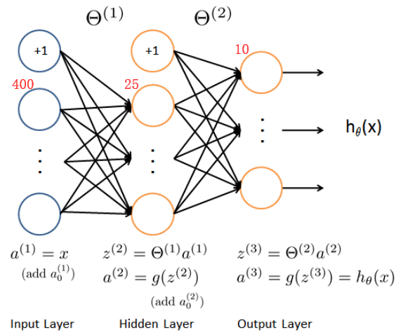
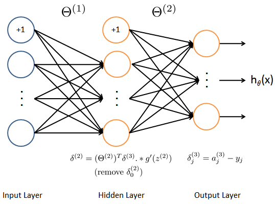
2 Feedforward and cost function 前馈和代价函数

确保每层的单元数，注意输出时加一个偏置单元，s(1)=400+1，s(2)=25+1，s(3)=10。

2.1 Sigmoid & forward Fuc

def sigmoid(z):
    return 1 / (1 + np.exp(-z))

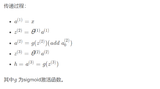
前馈传递过程

def forward(theta, X):
    '''得到每一层的输入和相关输出'''
    t1, t2 = deserialize(theta)
    # 前面已经插入过偏置单元，这里就不用插入了
    a1 = X
    z2 = a1 @ t1.T
    a2 = np.insert(sigmoid(z2), 0, 1, axis=1)
    # numpy.insert(arr,obj,value,axis=None)
    # value：插入的数值
    # arr：目标向量
    # obj：目标向量的axis维度的目标位置
    # axis ：为想要插入的维
    z3 = a2 @ t2.T
    a3 = sigmoid(z3)
    return a1, z2, a2, z3, a3

实现一下

a1, z2, a2, z3, h = forward(theta, X)

2.2 Cost Fuc

输出层输出的是对样本的预测，包含5000个数据，每个数据对应了一个包含10个元素的向量，代表了结果有10类。在公式中，每个元素与log项对应相乘。

def cost(theta, X, y):
    a1, z2, a2, z3, h = forward(theta, X)
    J = 0

    for i in range(len(X)):
        first = -y[i] * np.log(h[i])
        second = -(1 - y[i])*np.log(1 - h[i])
        J = J + sum(first + second)
        pass
    J = J/len(X)
    return J

向量化实现J

def cost2(theta, X, y):
    a1, z2, a2, z3, h = forward(theta, X)
    # or just use verctorization
    J = - y * np.log(h) - (1 - y) * np.log(1 - h)
    print(J.shape)      # (5000, 10)
    # 对应元素相乘
    return J, J.sum() / len(X)

a = cost(theta, X, y)       # 0.2876291651613187
J, b = cost2(theta, X, y)       # 0.2876291651613189
# print(a)

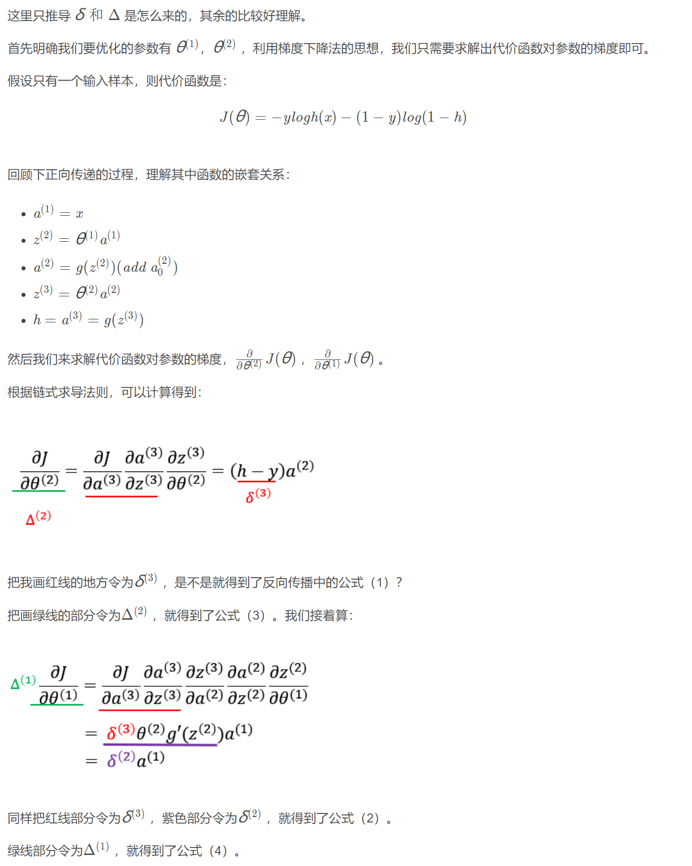
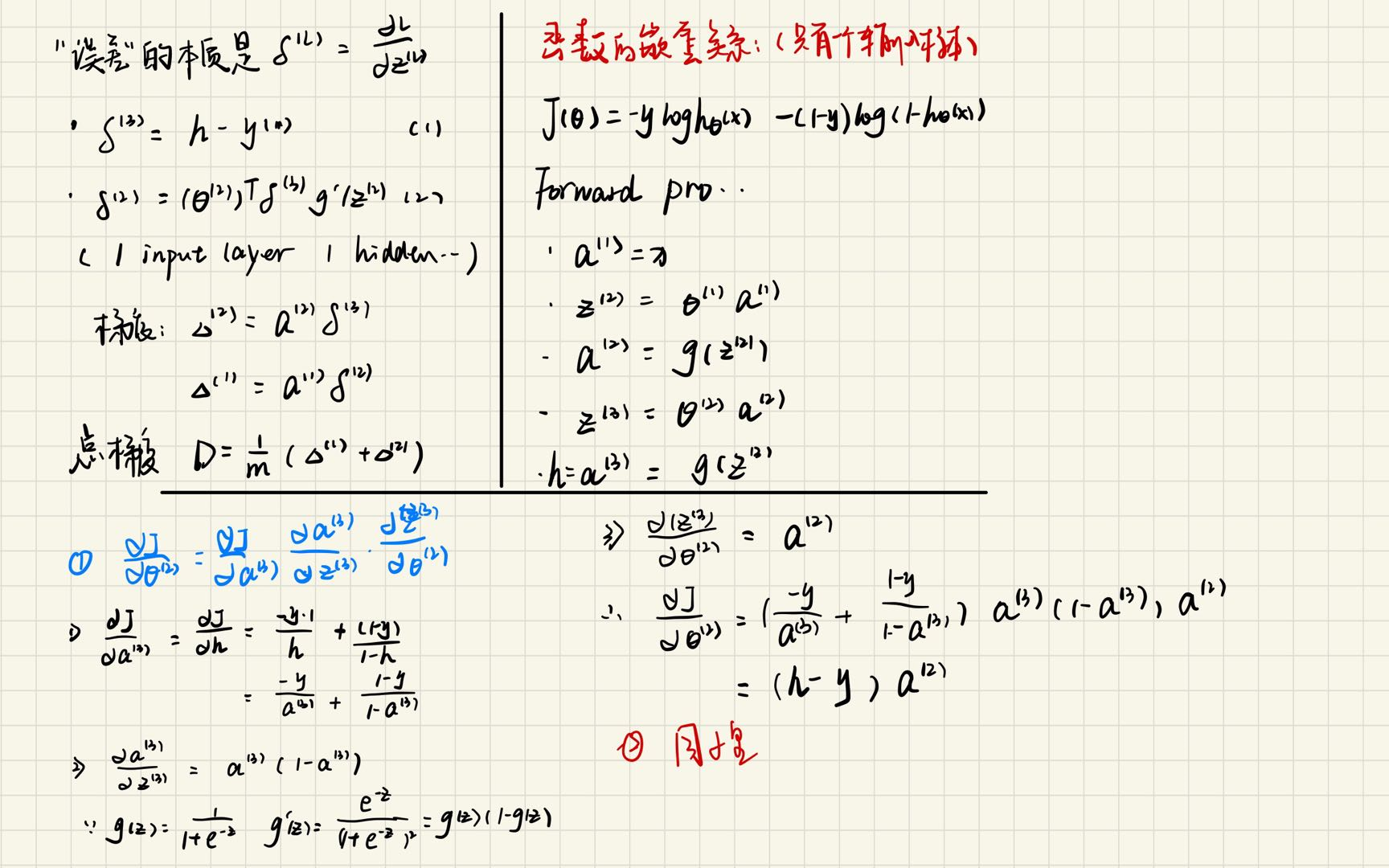
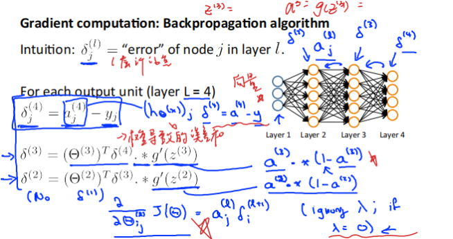
3 Backpropagation 反向传播

目标：获取整个网络代价函数的梯度。以便在优化算法中求解。

这里面一定要理解正向传播和反向传播的过程，才能弄清楚各种参数在网络中的维度，切记。比如手写出每次传播的式子。

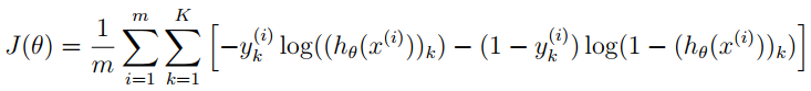
3.1 Regularized cost function 正则化代价函数

$$\begin{array}{rl}J(\theta )=& \frac{1}{m}\sum _{i=1}^m\sum _{k=1}^K\left[-y_k^{(i)}\log \left({\left(h_{\theta }\left(x^{(i)}\right)\right)}_k\right)-\left(1-y_k^{(i)}\right)\log \left(1-{\left(h_{\theta }\left(x^{(i)}\right)\right)}_k\right)\right]+\\ & \frac{\lambda }{2m}\left[\sum _{j=1}^{25}\sum _{k=1}^{400}{\left({\Theta }_{j,k}^{(1)}\right)}^2+\sum _{j=1}^{10}\sum _{k=1}^{25}{\left({\Theta }_{j,k}^{(2)}\right)}^2\right]\end{array}$$

注意不要将每层的偏置项正则化。

def regularized_cost(theta, X, y, lam):
    '''正则化时忽略每层的偏置项，也就是参数矩阵的第一列'''
    t1, t2 = deserialize(theta)
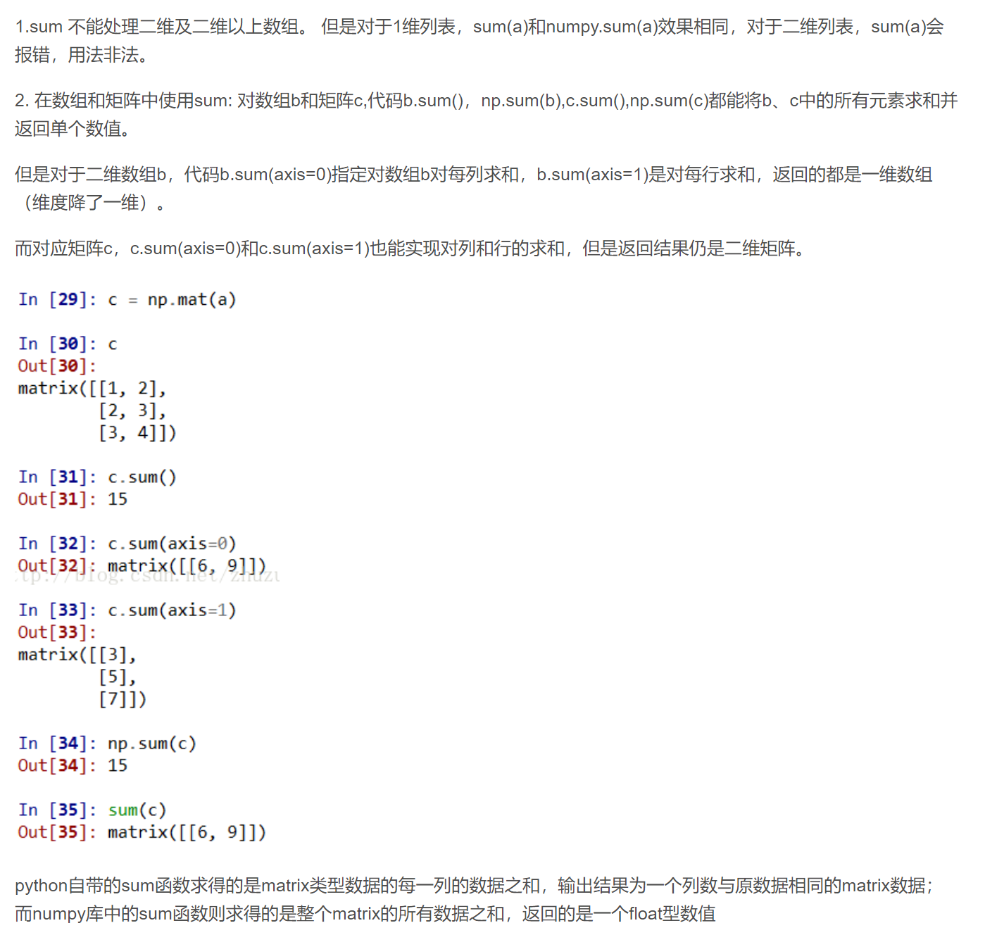
    # np.sum和sum的区别，前者是将所有的数都加起来，python自带的sum函数求得的是matrix类型数据的每一列的数据之和，
    # 输出结果为一个列数与原数据相同的matrix数据；而numpy库中的sum函数则求得的是整个matrix的所有数据之和，返回的是一个float型数值
    reg = np.sum(t1[:, 1:]**2) + np.sum(t2[:, 1:]**2)
    return lam/(2 * len(X)) * reg + cost(theta, X, y)

np.sum和sum的区别

costReg = regularized_cost(theta, X, y, 1)      # 0.3837698590909234

3.2 Regularized gradient function 正则化梯度下降函数

$$\begin{array}{ll}\frac{\partial }{\partial {\Theta }_{ij}^{(l)}}J(\Theta )=D_{ij}^{(l)}=\frac{1}{m}{\Delta }_{ij}^{(l)}& \text{ for }j=0\\ \frac{\partial }{\partial {\Theta }_{ij}^{(l)}}J(\Theta )=D_{ij}^{(l)}=\frac{1}{m}{\Delta }_{ij}^{(l)}+\frac{\lambda }{m}{\Theta }_{ij}^{(l)}& \text{ for }j\ge 1\end{array}$$

# sigmoid函数导数
def sigmoid_gradient(z):
    S = sigmoid(z)
    return S * (1-S)

def gradient(theta, X, y):
    '''
        unregularized gradient, notice no d1 since the input layer has no error
        return 所有参数theta的梯度，故梯度D(i)和参数theta(i)同shape，重要。
    '''
    t1, t2 = deserialize(theta)
    a1, z2, a2, z3, h = forward(theta, X)
    d3 = h - y  # (5000, 10)
    d2 = d3 @ t2[:, 1:] * sigmoid_gradient(z2)      # (5000, 25)
    D2 = d3.T @ a2      # (10, 26)
    D1 = d2.T @ a1      # (25, 401)
    D = (1 / len(X)) * serialize(D1, D2)        # (10285,)
    return D


def regularized_gradient(theta, X, y, lam):
    """不惩罚偏置单元的参数"""
    # a1, z2, a2, z3, h = forward(theta, X)
    D1, D2 = deserialize(gradient(theta, X, y))
    t1[:, 0] = 0
    t2[:, 0] = 0
    reg_D1 = D1 + (lam / len(X)) * t1
    reg_D2 = D2 + (lam / len(X)) * t2
    return serialize(reg_D1, reg_D2)

3.3 Random initialization 随机初始化

当我们训练神经网络时，随机初始化参数是很重要的，可以打破数据的对称性。
一个有效的策略是在均匀分布(−e，e)中随机选择值，我们可以选择 e = 0.12 这个范围的值来确保参数足够小，使得训练更有效率。

def random_init(size):
    '''从服从的均匀分布的范围中随机返回size大小的值,但是要接近0'''
    return  np.random.uniform(-0.12, 0.12, size)

print('a1', a1.shape,'t1', t1.shape)
print('z2', z2.shape)
print('a2', a2.shape, 't2', t2.shape)
print('z3', z3.shape)
print('a3', h.shape)
'''
a1 (5000, 401) t1 (25, 401)
z2 (5000, 25)
a2 (5000, 26) t2 (10, 26)
z3 (5000, 10)
a3 (5000, 10)
'''

3.4 Gradient checking 梯度检测

在你的神经网络,你是最小化代价函数J(Θ)。执行梯度检查你的参数,你可以想象展开参数Θ(1)Θ(2)成一个长向量θ。通过这样做,你能使用以下梯度检查过程。

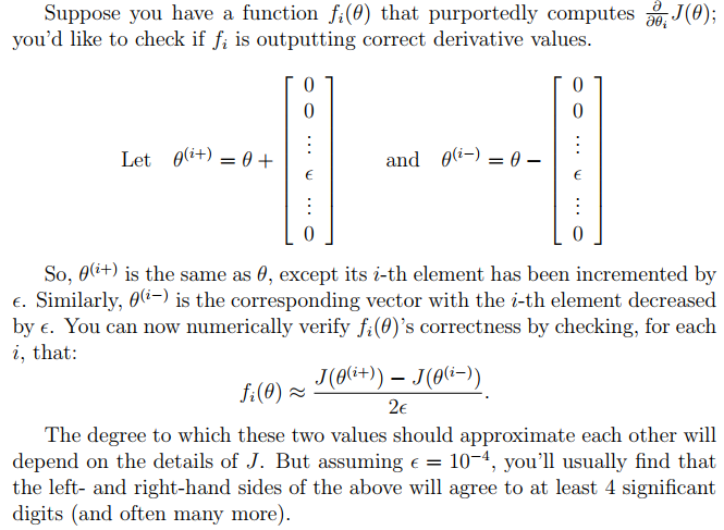
def gradient_checking(theta, X, y, e):
    def a_numeric_grad(plus, minus):
        """
        对每个参数theta_i计算数值梯度，即理论梯度。
        """
        return (regularized_cost(plus, X, y) - regularized_cost(minus, X, y)) / (e * 2)

    numeric_grad = []
    for i in range(len(theta)):
        plus = theta.copy()  # deep copy otherwise you will change the raw theta
        minus = theta.copy()
        plus[i] = plus[i] + e
        minus[i] = minus[i] - e
        grad_i = a_numeric_grad(plus, minus)
        numeric_grad.append(grad_i)

    numeric_grad = np.array(numeric_grad)
    analytic_grad = regularized_gradient(theta, X, y)
    diff = np.linalg.norm(numeric_grad - analytic_grad) / np.linalg.norm(numeric_grad + analytic_grad)

    print(
        'If your backpropagation implementation is correct,'
        '\nthe relative difference will be smaller than 10e-9 (assume epsilon=0.0001).'
        '\nRelative Difference: {}\n'.format(diff))
    pass

4 Training using fmincg

4.1 Learning parameters using fmincg 优化参数

def nn_training(X, y):
    init_theta = random_init(10285)     # 25*401 + 10*26
    res = opt.minimize(fun=regularized_cost, x0=init_theta, jac=regularized_gradient, method='TNC'
                       , options={'maxiter': 400}, args=(X, y, 1))
    return res

res = nn_training(X, y)
print(res)

'''
 fun: 0.4925270115328131
     jac: array([-1.05190454e-03, -2.11248326e-12,  4.38829369e-13, ...,
       -2.04581092e-03, -1.92890884e-03, -1.72523053e-03])
 message: 'Converged (|f_n-f_(n-1)| ~= 0)'
    nfev: 380
     nit: 19
  status: 1
 success: True
       x: array([ 0.7801655 ,  0.07875929, -0.1014434 , ...,  0.70208755,
        3.70930944, -2.03648228])
'''

def accyracy(theta, X, y):
    _, _, _, _, h = forward(theta, X)
    # np.nanargmax(a)
    # 返回Nan之外的最大值的索引
    y_pred = np.nanargmax(h, axis=1) + 1    # 找到概率最大的并返回值为col_index+1, axis=1 意味着只返回列的
    print(classification_report(y, y_pred))
    return y_pred, h

y_pred, h = accyracy(res.x, X, raw_y)
print(h)
'''
             precision    recall  f1-score   support
           1       0.97      0.99      0.98       500
           2       0.98      0.96      0.97       500
           3       0.98      0.95      0.96       500
           4       0.98      0.98      0.98       500
           5       0.98      0.98      0.98       500
           6       0.98      0.99      0.98       500
           7       0.98      0.97      0.97       500
           8       0.97      0.99      0.98       500
           9       0.97      0.97      0.97       500
          10       0.98      1.00      0.99       500
    accuracy                           0.98      5000
   macro avg       0.98      0.98      0.98      5000
weighted avg       0.98      0.98      0.98      5000

'''

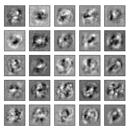
4.2 Visualizing the hidden layer 可视化隐藏层

理解神经网络是如何学习的一个很好的办法是, 可视化隐藏层单元所捕获的内容。通俗的说，给定一个的隐藏层单元，可 视化它所计算的内容的方法是找到一个输入 $x,x$ 可以激活这个单元 (也就是说有一个激活值 $a_i^{(l)}$ 接近与1) 。对于我们所 训练的网络, 注意到01中每一行都是一个401维的向量，代表每个隐藏层单元的参数。如果我们忽略偏置项, 我们就能得 到400维的向量，这个向量代表每个样本输入到每个隐层单元的像素的权重。因此可视化的一个方法是, reshape这个400 维的向量为 $(20,20)$ 的图像然后输出。

def plot_hidden(theta):
    t1, _ = deserialize(theta)
    t1 = t1[:, 1:]
    fig, ax_array = plt.subplots(5, 5, sharex=True, sharey=True, figsize=(6, 6))
    for r in range(5):
        for c in range(5):
            ax_array[r, c].matshow(t1[r * 10 + c].reshape(20, 20), cmap='gray_r')
            plt.xticks([])
            plt.yticks([])
            pass
        pass
    plt.show()
    pass

plot_hidden(res.x)

文末附有所有的代码

import numpy as np
import matplotlib.pyplot as plt
from scipy.io import loadmat
import scipy.optimize as opt
from sklearn.metrics import classification_report  # 这个包是评价报告
from sklearn.preprocessing import OneHotEncoder

'''
1.Prepare datasets
'''


def load_mat(path):
    '''
    读取数据
    :param path:
    :return:
    '''
    data = loadmat(path)
    X = data['X']
    y = data['y'].flatten()
    return X, y


def plot_100_image(X):
    '''
    随机画100个数字
    :return:
    '''
    inedx = np.random.choice(range(5000), 100)
    images = X[inedx]
    fig, ax_array = plt.subplots(10, 10, sharex=True, sharey=True, figsize=(8, 8))
    for r in range(10):
        for c in range(10):
            ax_array[r, c].matshow(images[r*10 + c].reshape(20, 20), cmap='gray_r')
            pass
        pass
    plt.xticks([])
    plt.yticks([])
    plt.show()
    pass


# Visualizing the data
# X, y = load_mat('ex4data1.mat')
# plot_100_image(X)


'''
2.Neural model representation   神经网络模型展示
'''

# 2.1 Load train dataset
'''
首先我们要将标签值（1，2，3，4，…，10）转化成非线性相关的向量，向量对应位置（y[i-1]）上的值等于1，
例如y[0]=6转化为y[0]=[0,0,0,0,0,1,0,0,0,0]。
'''


def expand_y(y):
    result = []
    # 把y中每个类别转化为一个向量，对应的lable值在向量对应位置上置为1
    # 从0开始计数
    for i in y:
        y_array = np.zeros(10)
        y_array[i-1] = 1
        result.append(y_array)
    '''
    # 或者用sklearn中OneHotEncoder函数
    encoder =  OneHotEncoder(sparse=False)  # return a array instead of matrix
    y_onehot = encoder.fit_transform(y.reshape(-1,1))
    return y_onehot
    '''
    return np.array(result)


# a = expand_y(y)

raw_X, raw_y = load_mat('ex4data1.mat')
X = np.insert(raw_X, 0, 1, axis=1)
y = expand_y(raw_y)
print(X.shape, y.shape)     # (5000, 401), (5000, 10)


# 2.2 Load weights
# 这里我们提供了已经训练好的参数θ1，θ2，存储在ex4weight.mat文件中。
# 这些参数的维度由神经网络的大小决定，第二层有25个单元，输出层有10个单元(对应10个数字类)。
def load_weights(path):
    data = loadmat(path)
    return data['Theta1'], data['Theta2']


t1, t2 = load_weights('ex4weights.mat')
print(t1.shape, t2.shape)   # (25, 401) (10, 26)


# 2.3 展开参数
# 当我们使用高级优化方法来优化神经网络时，我们需要将多个参数矩阵展开，才能传入优化函数，然后再恢复形状。
def serialize(a, b):
    '''
    展开参数
    np.r_是按列连接两个矩阵，就是把两矩阵上下相加，要求列数相等。
    np.c_是按行连接两个矩阵，就是把两矩阵左右相加，要求行数相等。
    '''
    return np.r_[a.flatten(), b.flatten()]


theta = serialize(t1, t2)   # 扁平化参数，25*401+10*26=10285
print(theta.shape)      # (10285,)


def deserialize(seq):
    '''提取参数'''
    return seq[:25*401].reshape(25, 401), seq[25*401:].reshape(10, 26)


'''
3.Feedforward and cost function 前馈和代价函数
'''


def sigmoid(z):
    return 1 / (1 + np.exp(-z))


def forward(theta, X):
    '''得到每一层的输入和相关输出'''
    t1, t2 = deserialize(theta)
    # 前面已经插入过偏置单元，这里就不用插入了
    a1 = X
    z2 = a1 @ t1.T
    a2 = np.insert(sigmoid(z2), 0, 1, axis=1)
    # numpy.insert(arr,obj,value,axis=None)
    # value：插入的数值
    # arr：目标向量
    # obj：目标向量的axis维度的目标位置
    # axis ：为想要插入的维
    z3 = a2 @ t2.T
    a3 = sigmoid(z3)
    return a1, z2, a2, z3, a3


a1, z2, a2, z3, h = forward(theta, X)


def cost(theta, X, y):
    a1, z2, a2, z3, h = forward(theta, X)
    J = 0

    for i in range(len(X)):
        first = -y[i] * np.log(h[i])
        second = -(1 - y[i])*np.log(1 - h[i])
        J = J + sum(first + second)
        pass
    J = J/len(X)
    return J

# 向量化实现J
def cost2(theta, X, y):
    a1, z2, a2, z3, h = forward(theta, X)
    # or just use verctorization
    J = - y * np.log(h) - (1 - y) * np.log(1 - h)
    print(J.shape)      # (5000, 10)
    # 对应元素相乘
    return J, J.sum() / len(X)


a = cost(theta, X, y)       # 0.2876291651613187
J, b = cost2(theta, X, y)       # 0.2876291651613189
# print(a)
'''
4.Regularized cost function 正则化代价函数
'''


def regularized_cost(theta, X, y, lam):
    '''正则化时忽略每层的偏置项，也就是参数矩阵的第一列'''
    t1, t2 = deserialize(theta)
    # np.sum和sum的区别，前者是将所有的数都加起来，python自带的sum函数求得的是matrix类型数据的每一列的数据之和，
    # 输出结果为一个列数与原数据相同的matrix数据；而numpy库中的sum函数则求得的是整个matrix的所有数据之和，返回的是一个float型数值
    reg = np.sum(t1[:, 1:]**2) + np.sum(t2[:, 1:]**2)
    return lam/(2 * len(X)) * reg + cost(theta, X, y)


costReg = regularized_cost(theta, X, y, 1)      # 0.3837698590909234
'''
5.Backpropagation 反向传播
'''


# sigmoid函数导数
def sigmoid_gradient(z):
    S = sigmoid(z)
    return S * (1-S)


# Random initialization 随机初始化
# 当我们训练神经网络时，随机初始化参数是很重要的，可以打破数据的对称性。
# 一个有效的策略是在均匀分布(−e，e)中随机选择值，我们可以选择 e = 0.12 这个范围的值来确保参数足够小，使得训练更有效率。
def random_init(size):
    '''从服从的均匀分布的范围中随机返回size大小的值,但是要接近0'''
    return  np.random.uniform(-0.12, 0.12, size)


print('a1', a1.shape,'t1', t1.shape)
print('z2', z2.shape)
print('a2', a2.shape, 't2', t2.shape)
print('z3', z3.shape)
print('a3', h.shape)
'''
a1 (5000, 401) t1 (25, 401)
z2 (5000, 25)
a2 (5000, 26) t2 (10, 26)
z3 (5000, 10)
a3 (5000, 10)
'''


def gradient(theta, X, y):
    '''
        unregularized gradient, notice no d1 since the input layer has no error
        return 所有参数theta的梯度，故梯度D(i)和参数theta(i)同shape，重要。
    '''
    t1, t2 = deserialize(theta)
    a1, z2, a2, z3, h = forward(theta, X)
    d3 = h - y  # (5000, 10)
    d2 = d3 @ t2[:, 1:] * sigmoid_gradient(z2)      # (5000, 25)
    D2 = d3.T @ a2      # (10, 26)
    D1 = d2.T @ a1      # (25, 401)
    D = (1 / len(X)) * serialize(D1, D2)        # (10285,)
    return D


def regularized_gradient(theta, X, y, lam):
    """不惩罚偏置单元的参数"""
    # a1, z2, a2, z3, h = forward(theta, X)
    D1, D2 = deserialize(gradient(theta, X, y))
    t1[:, 0] = 0
    t2[:, 0] = 0
    reg_D1 = D1 + (lam / len(X)) * t1
    reg_D2 = D2 + (lam / len(X)) * t2
    return serialize(reg_D1, reg_D2)


'''
6.Gradient checking 梯度检测
'''


def gradient_checking(theta, X, y, e):
    def a_numeric_grad(plus, minus):
        """
        对每个参数theta_i计算数值梯度，即理论梯度。
        """
        return (regularized_cost(plus, X, y) - regularized_cost(minus, X, y)) / (e * 2)

    numeric_grad = []
    for i in range(len(theta)):
        plus = theta.copy()  # deep copy otherwise you will change the raw theta
        minus = theta.copy()
        plus[i] = plus[i] + e
        minus[i] = minus[i] - e
        grad_i = a_numeric_grad(plus, minus)
        numeric_grad.append(grad_i)

    numeric_grad = np.array(numeric_grad)
    analytic_grad = regularized_gradient(theta, X, y)
    diff = np.linalg.norm(numeric_grad - analytic_grad) / np.linalg.norm(numeric_grad + analytic_grad)

    print(
        'If your backpropagation implementation is correct,'
        '\nthe relative difference will be smaller than 10e-9 (assume epsilon=0.0001).'
        '\nRelative Difference: {}\n'.format(diff))
    pass


'''
7.Learning parameters using fmincg 优化参数
'''


def nn_training(X, y):
    init_theta = random_init(10285)     # 25*401 + 10*26
    res = opt.minimize(fun=regularized_cost, x0=init_theta, jac=regularized_gradient, method='TNC'
                       , options={'maxiter': 400}, args=(X, y, 1))
    return res


res = nn_training(X, y)
print(res)
'''
 fun: 0.4925270115328131
     jac: array([-1.05190454e-03, -2.11248326e-12,  4.38829369e-13, ...,
       -2.04581092e-03, -1.92890884e-03, -1.72523053e-03])
 message: 'Converged (|f_n-f_(n-1)| ~= 0)'
    nfev: 380
     nit: 19
  status: 1
 success: True
       x: array([ 0.7801655 ,  0.07875929, -0.1014434 , ...,  0.70208755,
        3.70930944, -2.03648228])
'''


def accyracy(theta, X, y):
    _, _, _, _, h = forward(theta, X)
    # np.nanargmax(a)
    # 返回Nan之外的最大值的索引
    y_pred = np.nanargmax(h, axis=1) + 1    # 找到概率最大的并返回值为col_index+1, axis=1 意味着只返回列的
    print(classification_report(y, y_pred))
    return y_pred, h

y_pred, h = accyracy(res.x, X, raw_y)
print(h)
'''
             precision    recall  f1-score   support
           1       0.97      0.99      0.98       500
           2       0.98      0.96      0.97       500
           3       0.98      0.95      0.96       500
           4       0.98      0.98      0.98       500
           5       0.98      0.98      0.98       500
           6       0.98      0.99      0.98       500
           7       0.98      0.97      0.97       500
           8       0.97      0.99      0.98       500
           9       0.97      0.97      0.97       500
          10       0.98      1.00      0.99       500
    accuracy                           0.98      5000
   macro avg       0.98      0.98      0.98      5000
weighted avg       0.98      0.98      0.98      5000

'''


def plot_hidden(theta):
    t1, _ = deserialize(theta)
    t1 = t1[:, 1:]
    fig, ax_array = plt.subplots(5, 5, sharex=True, sharey=True, figsize=(6, 6))
    for r in range(5):
        for c in range(5):
            ax_array[r, c].matshow(t1[r * 5 + c].reshape(20, 20), cmap='gray_r')
            plt.xticks([])
            plt.yticks([])
            pass
        pass
    plt.show()
    pass


plot_hidden(res.x)

参考链接：https://blog.csdn.net/Cowry5/article/details/80367832